Ultrasound Probe Element Dropout: The Line, the Test, the Threshold
Same symptom on your system?
Tell us your model and what it is doing. A GEPROBE engineer replies with a diagnosis path, part options and pricing — usually within 6 hours, with no obligation.
Chat on WhatsApp
The position of the line is the argument
A dark band that belongs to an array element behaves in one specific way: it keeps its place relative to the probe face. Move the probe across the body, change the preset, add gain, add coupling gel, and the band does not follow the tissue underneath it. It stays at the same lateral position, scan after scan. That behaviour carries most of the argument. Anatomy moves with the probe. A disturbance at the contact surface — a bubble, a fold of gel, a scarred lens — moves and changes shape with the surface it sits on. An element cannot, because it occupies a fixed position in the array.
The signature can be produced without any test equipment at all. With the probe held in air and no gel, the impedance mismatch between the lens and the air returns a stack of horizontal reverberation bands across the image. A dead or weak element cuts a vertical stripe through those bands; a delaminated lens distorts them more broadly. Automated analysis of that pattern has been validated as a screening method, and the same view underpins the five-year quality assurance programme discussed further down this page. For phased arrays operated in M-mode, the element-test literature describes the defect as a dark axial band appearing at the position of the failed element. A thin metal rod drawn slowly across the face through a little gel reproduces the effect element by element; the published version of the method uses a 0.73 mm rod.
What the morphology will not do is name a cause. A fine shadow on one channel and a wide shadow across a contiguous block are different findings, and neither of them tells you whether the broken link is a crystal, an adhesive layer, a wire in the cable, or a channel on the far side of the connector. Three quite different failures produce very nearly the same picture.
This page is written for the people who own the probe rather than the people scanning with it — clinical engineering, equipment departments, and whoever has to sign for a replacement. It is not a repair procedure, and it is not clinical guidance: the measurements below describe what a probe is doing, not how any examination should be interpreted.
The same line, four owners
Four things produce that band. A multicentre survey of probes in clinical use found a fault in more than one in three of them, and an earlier study of 676 probes that ran the same instruments through an electronic tester resolved the faults into categories: delamination 67%, cable faults 30%, dead or weak elements 4%. The band on the display is the least common of the three, and it is the one with the shortest list of mechanisms behind it.
| Appearance in the image | What it most often is | The move that separates it |
|---|---|---|
| Fine single-channel shadow, stable | A single element, or its bond to the flex circuit | Per-element electrical test; the band does not change when the cable is flexed |
| Wider shadow across several channels | A block of elements, or a delaminated lens sitting over intact crystals | In-air reverberation plus a per-element test, and a physical look at the lens |
| Band that flickers, narrows or disappears as the cable is flexed | Interconnect or a cable conductor, not the array | Flex the cable section by section while watching a uniform image |
| Band that stays on the same port when a known-good probe is connected | System side: a front-end channel or the connector | Swap probes; inspect the pin bank for bent or corroded pins |
The last row is the one that changes budgets. The same stripe can be manufactured on the system side of the connector, and front-end or connector faults are not probe faults: no amount of probe work removes them. That is why the published physical-inspection guides put the connector pin bank in the same list as the lens, the housing, the strain relief and the cable — the connector is the one place where a probe fault and a system fault look alike.
The isolation sequence is short. Connect a known-good probe to the port that produced the band. If the band is gone, the probe is implicated; if it is still there, the port is. Then put the suspect probe on a second port to confirm. Then, for any band that is not rock steady, flex the cable in three sections — behind the probe-end strain relief, mid-cable, and at the connector end — while a uniform image is on screen. A band that moves with the flexion is a conductor problem, and it belongs to the cable end of the probe rather than the array. That last behaviour is a small case of a much wider discipline: faults that will not reproduce while an engineer is watching follow their own rules, and intermittent ultrasound faults are worked through separately. The console side of the same question — proving the system is not the variable before the probe is blamed — is the discipline that sits behind checking the console before the probe, and it applies whether the probe is being bought or repaired.
Once the fault is localised to the probe, the question stops being diagnostic and becomes one of supply or repair, and the probe catalogue lists what we hold for that. No price appears on this page, and nothing here promises that any particular probe can be brought back to specification — only a measurement taken on that instrument can say so.
What each test reads, and what it takes to run
Four methods are in routine use, and they do not answer the same question. What separates them is not sophistication but the physical quantity each one actually reads.
| Test | The quantity it reads | How fine it resolves | What has to be available |
|---|---|---|---|
| In-air reverberation | Uniformity and sensitivity along the array, from the lens-to-air mismatch | A single element, given the right settings and a clean lens | Nothing beyond the system itself |
| Electronic element tester | Per-element sensitivity and capacitance, and continuity of the wiring | One element at a time, with a position for each | The tester and a probe-specific adapter |
| Tissue-mimicking phantom | Gross uniformity, penetration, geometric accuracy | Poorly, for small or non-adjacent blocks | Phantom, fixed settings, a consistent operator |
| Physical inspection | Lens, housing, strain reliefs, cable, connector pin bank | Not at all — the electronics are never interrogated | Light, magnification, a written list |
The expectation that an ultrasound system carry an element check is not a local preference. The FDA's guidance on diagnostic ultrasound systems and transducers, issued in final form in February 2023 and originally published in June 2019, devotes a section to the transducer element check: each device should include some level of testing, and the guidance offers an impedance check of each transducer element as the example, noting that this is a preliminary evaluation of element integrity and function. The same section expects the integrated test to be available to operators when a probe is suspected of failure.
What that looks like on a specific platform is documented in the quick card for the GE Vivid iq: the test is reached from Probe and then Preset Config and Test Probe, a failing result raises a reminder window, and the probe-check interval itself is configurable. One operational note in that card is easy to skip past — the probe lens should be clean during the test, because gel residue can affect the result. An element check with a contaminated face is a test with an uncontrolled variable.
A built-in check is a gate, not a report. In a comparison of three quality assurance methods for clinical ultrasound devices, the manufacturer's own internal transducer test could not be used at all, because it was not available on every system included in the study; the element-resolved answer had to come from an independent tester or from the in-air image. The free method has an unusual amount of published mileage behind it: one programme tested 21 transducers every other month for five years, an average of 11.7 tests per transducer, at about 2.75 hours of testing labour per transducer per year, and recorded a mean annual fail rate of 10.7%.
The threshold the tester prints
An electronic tester turns sensitivity into a number per element, and the classification published alongside one of those instruments is worth reproducing because it is what the term "dead element" actually means in a report. An element operating below 10% of the highest-sensitivity element in the array is classed as dead. An element between 10% and 40% of the array mean is weak. An element at or above 75% of the mean is intact, and the band between 40% and 75% is classed as acceptable. Defective, in that scheme, is the union of the weak and malfunctioning groups.
Two things about those bands matter more than the numbers themselves. The first is that a reading below the dead threshold does not identify a dead element. The same documentation gives four candidates for a sensitivity that low: a dead element, an open cable, a broken connector pin, or lens delamination. The instrument prints amplitudes; a person decides which of the four mechanisms is behind them. The second is that the bands belong to the tester's user guide and were adopted as a starting point by later published comparisons. They are not a standard, the manufacturers are not obliged to use them, and the same probe can sit acceptably on one side of a threshold for one intended use and not for another — which is why the intended use has to be in the room when the classification is.
The trade names cited on this page — the testers, the platforms, and their menus — belong to their respective owners. We are not affiliated with any of them. They appear here as the origin of a published figure or a documented procedure, and for no other reason.
Why the count is the wrong currency
The useful unit is not how many elements are gone. It is where they are and whether they are next to each other, and the measurements behind that statement are unusually concrete. A study in the Journal of Diagnostic Medical Sonography disabled selected elements on working arrays and then measured the beams: as few as two dead elements sitting side by side changed the beam profile, pushing energy into the side lobes and costing signal-to-noise, and on one array the transmitted acoustic output fell from 88 mW/cm² (SPTA) to 73 mW/cm² (SPTA). On a 128-element array with six dead elements in a row, the same work recorded a fall from roughly 103 to roughly 67 mW/cm². A separate measurement reported in a five-year quality assurance programme found a 33% reduction in Doppler flow when six elements were disabled, and the same study points out that dead elements show up in Doppler as peak-velocity errors and flow ambiguity rather than as an obvious defect.
The mechanism is worth stating because it explains why position carries the weight. The beam width at the focus is set by the active aperture through the f-number, so removing a contiguous block of elements narrows the aperture and moves energy out of the main lobe into the side lobes. On receive, each element feeds its own channel and its own converter, so the array's summation gain falls as channels drop out — the loss is not proportional to the count alone, it is a loss of processing gain on top of a loss of aperture.
Position matters in a second, less intuitive way. Non-adjacent non-functioning elements can raise grating lobes sharply, because an array with holes in it is no longer a uniformly weighted periodic structure. A phantom uniformity measurement can report identical coupling for every element while the beam has already changed, and a probe with two scattered dead elements can measure worse than a probe with the same number of elements missing in one place — or better, depending on where the place is. Tissue-mimicking phantoms, the same study concluded, are equivocal at best at detecting dead elements, which is exactly what one would expect from a test that averages over the aperture the defects are sitting in.
Put together, this is why a report that prints a count of dead elements, without saying which elements, cannot carry the decision it is usually quoted for.
Where the tests disagree with each other
The methods do not merely differ in resolution; they disagree on individual probes. In one comparison of 37 probes measured with all three methods, the electronic tester and the in-air view agreed on functional-versus-defective in 86.5% of cases, as did the uniformity test and the in-air view, leaving a 21.6% mismatch between methods overall. The tester identified six transducers as malfunctioning that the phantom uniformity test had called normal. One probe read intact under both the tester and the uniformity test and defective under the in-air image.
The in-air view also has a known geometry problem. On a 3D mechanical transducer, two non-consecutive dead elements did not appear as signal loss in the reverberation profile at all, because in that design the elements are steered rather than fixed to a single row; the authors' caution is that losses in a mechanical 3D probe can be underestimated by that test. And there is no agreed standard for how the in-air pattern should look at acceptance, which is why a same-model reference probe and a recorded baseline end up doing work that a published threshold cannot do.
Frequency is the other disagreement. An annual check reads like a reasonable interval until it is measured: 299 probes re-tested a year after an earlier survey produced 81 defective instruments, 27.1% of the sample, and the failing group included probes that had passed the previous round and probes that had been bought to replace failures. The paper that reports this is titled, without much hedging, "Ultrasound transducer function: annual testing is not sufficient."
Underneath all of it sits the least objective step in the chain. Phantom-based visual assessment, in the comparison of the three methods, was the least objective of them, and the beam-profile literature makes the same point from the other side: small differences in contrast and resolution in a speckle image can only be recognised by highly experienced observers. A test whose pass mark is "nothing obvious today" is not a test with a number in it.
Repair, replace, or keep watching
Acceptance testing is where all of this stops being an engineering curiosity and becomes a document. In a five-year acceptance programme that applied the in-air view to every probe delivered to an organisation, 233 new probes arrived and 13.7% of them had anomalous reverberation patterns; the conclusion the authors draw is worth carrying as a rule. A probe showing dropout should not be accepted into clinical use, and where the reverberation lines are not parallel the probe should be rejected unless the supplier can show that sensitivity, uniformity and bandwidth are unaffected.
The same rule read backwards gives the three-way fork for a probe already in the field, and the measurement decides which branch it takes. One weak element, isolated, on a probe whose intended work never uses that part of the sector: keep it in service and shorten the interval between tests, because 27.1% of a re-tested sample had become defective within a year. A contiguous block of dead elements, or any dropout on a probe used for Doppler: the beam profile evidence above puts that in the repair-or-replace branch, not the monitoring one — six disabled elements cost a third of the Doppler flow in the measurement cited earlier. A reading the tester calls dead that disappears when the probe is moved to another port: the fork is not about the probe at all, and the fault is on the system side.
Whatever branch a probe lands in, the report behind the decision will be read again in a year, and the fields that keep it usable are few:
- the method, named — because the methods disagree with each other on 21.6% of probes;
- the reference the comparison was made against, a threshold or a same-model probe, since the in-air pattern has no agreed standard;
- per-element results with positions, since contiguity decides more than the count;
- the date, the settings and the lens condition, because the only meaningful comparison is against the instrument's own earlier number.
The measurement is not the verdict. Nothing on this page states a price, and nothing on it promises that a given probe will be restored to specification: the thresholds above belong to the tester that publishes them, the failure rates belong to the programmes that measured them, and the only statement about a specific probe is the one that instrument's own test supports.
Which returns the argument to where it started. The fault that makes the most legible mark on the screen — one dark line, fixed in place, impossible to mistake for anything else — is the least common of the three main probe faults, and it is the easiest one to attribute. Delamination and cable faults, which between them made up the rest of what the surveys counted, come with no such convenient geometry, and they are why a probe passed as normal two hours ago can be inside the re-test group a year from now. A dropout line is the visible case. The rest of the page is about the ones that are not visible, and about the fact that the only way to rank them is to measure the array element by element and keep the numbers.
Related Articles
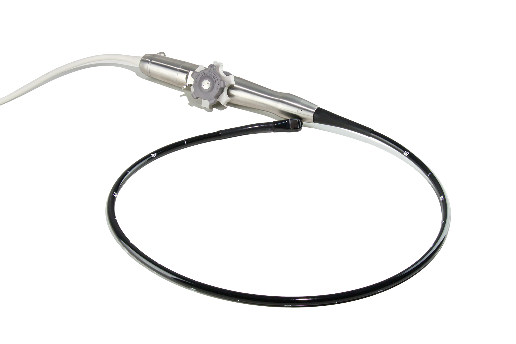
Ultrasound Probe Leakage Current: The Limit Depends on the Condition
A probe can image perfectly and still fail its electrical safety test. The limit a leakage reading is judged against changes with the probe's applied-part class, the grounding condition and the mains voltage, and the manufacturer's own tables say so.
Array Probe Pitch: It Sets Steering Range, Not Resolution
Pitch is the centre-to-centre distance between array elements — the sum of element width and kerf. It is not the number that sets resolution. It is the number that decides how far a beam can be steered before a second, equally strong lobe appears somewhere it was not aimed.
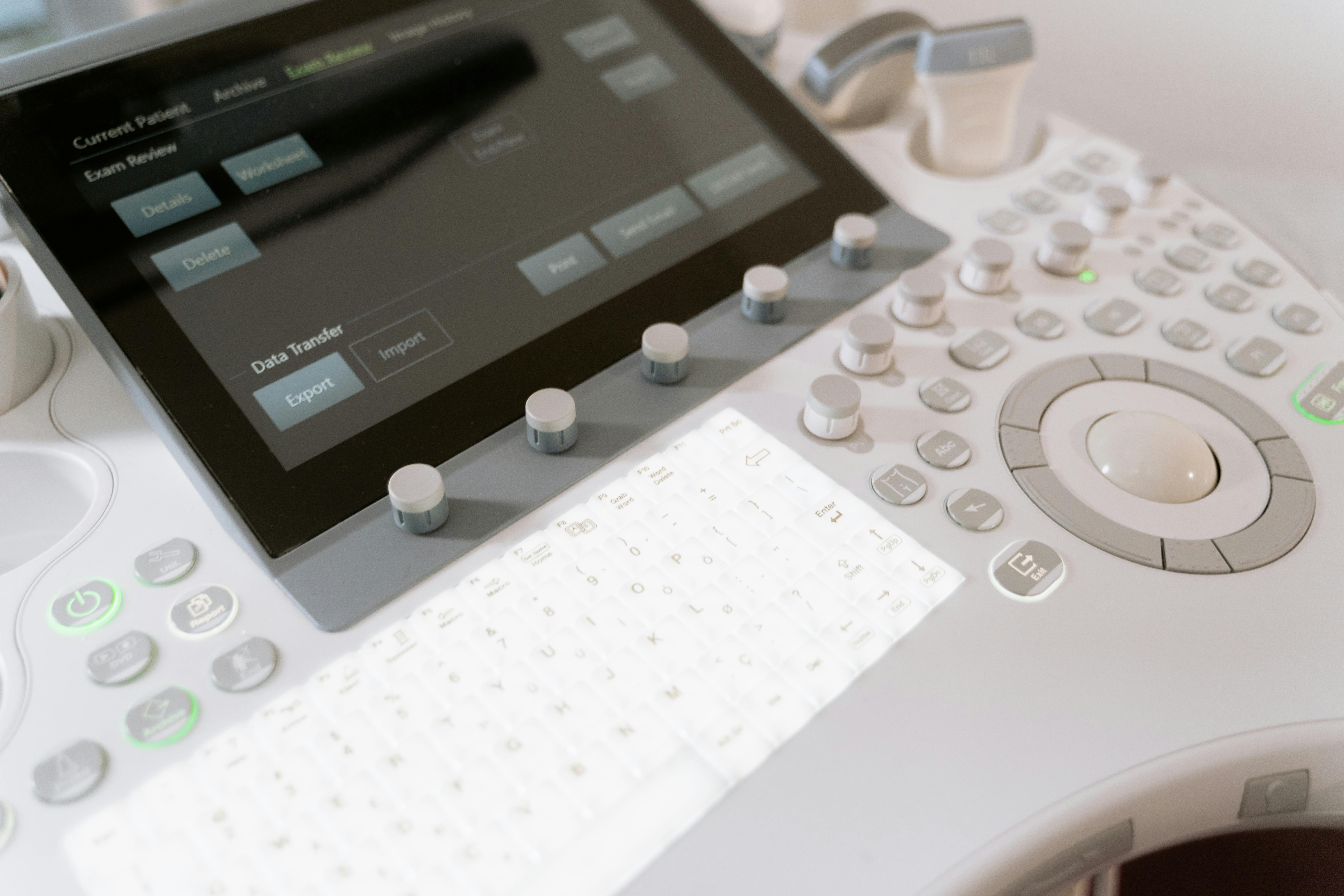
GE VIVID E9 Touch Screen Calibration: Which Routine, and When
The VIVID E9 service manual prints the same first remedy for a touch panel that activates the wrong control and for one that stops answering. What the calibration dialog moves, where the system's other calibration lives, and what the escalation order is really covering.